How to Make Subscript in Excel: A Complete Guide

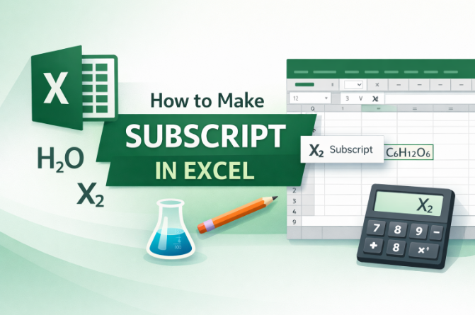
When working with data in Microsoft Excel, proper formatting is crucial to ensure that your content is visually appealing and easy to understand. One such formatting option is the ability to apply subscript to text or numbers within cells. Subscripts are typically used in mathematical formulas, chemical equations, or any situation where you need to display characters at a smaller size and slightly lower than the rest of the text. In this comprehensive guide, we will explore various methods to make subscript in Excel.

Understanding Subscript in Excel

Before we dive into the specific methods, let’s first understand what subscript formatting is. Subscript refers to text that appears smaller than the rest of the characters, usually positioned slightly below the normal line of text. This is often used for:

• Chemical formulas (e.g., H₂O)
• Mathematical expressions (e.g., x²)
• Footnotes or references in academic papers

In Excel, subscript formatting is available for both numbers and letters. However, the method to apply subscript formatting varies depending on whether you’re working with an individual cell, a part of a cell’s content, or an entire formula. Let’s explore these methods in detail.

Method 1: Using the Format Cells Dialog Box to Make Subscript in Excel

One of the simplest ways to apply subscript formatting is through the Format Cells dialog box. This method works when you want to apply subscript to entire numbers or text in a cell.

Steps:

1. Select the cell where you want to apply the subscript. For example, click on the cell containing the text or number you want to format.
2. Right-click the selected cell and choose Format Cells from the context menu, or you can also press Ctrl + 1 on your keyboard as a shortcut.
3. In the Format Cells dialog box, navigate to the Font tab.
4. Under the Effects section, you will see an option for Subscript. Check the Subscript box.
5. Click OK to apply the changes. The content in the selected cell will now appear as subscript.

Example:
If you have a cell with the text “H2O,” applying the subscript effect will transform it into “H₂O,” where the “2” is formatted as a subscript.

Read more: How to Make Subscript in Excel

Method 2: Using the Keyboard Shortcut

For those who prefer working quickly without navigating through menus, Excel offers a keyboard shortcut that allows you to toggle subscript formatting on and off. This method is particularly useful for making quick adjustments within a cell.

Steps:

1. Click on the cell that contains the text or numbers you want to format.
2. Highlight the specific part of the text that you want to make subscript. If you want to apply subscript to the entire cell content, simply click on the cell.
3. Press Ctrl + = on your keyboard. This shortcut will toggle the subscript formatting for the selected text or number.
4. Press the same combination again to remove the subscript formatting if needed.

Example:
To make “x²” appear as “x₂” with the “2” in subscript, simply select the “2” and press Ctrl + =.

Method 3: Using the Ribbon to Make Subscript in Excel

Excel’s Home ribbon also provides a quick way to format text as subscript. This method can be useful when you need to apply subscript formatting to parts of the cell’s contents without going through the context menu or using keyboard shortcuts.

Steps:

1. Select the cell that contains the text you want to format.
2. Highlight the part of the text or number that you want to make subscript.
3. Go to the Home tab on the Excel ribbon.
4. In the Font group, you will find the Subscript button (it looks like an “x” with a small “2” below it).
5. Click the Subscript button, and the highlighted text will be formatted as subscript.

Example:
If your cell contains the text “C6H12O6” and you want to make the “6”s subscript, select the “6”s, and click the Subscript button on the ribbon.

Method 4: Using the Rich Text Format in Excel Cells

In some cases, you may need to make subscript in Excel, formatting to only a portion of the text within a single cell, especially when the cell contains both normal text and subscripted content. Excel allows you to format individual parts of a cell’s content by using the Rich Text feature.

Steps:

1. Double-click the cell where you want to apply subscript formatting.
2. Select the part of the text that you want to make subscript.
3. Right-click the selected text and choose Format Cells, or go to the Home tab and select the Font dropdown.
4. Check the Subscript option in the Format Cells dialog box, then click OK.
5. The selected part of the text will now be formatted as subscript, while the rest of the text remains unchanged.

Example:
If you have “2H2O” in a cell and you only want the “2” after H and O to appear as subscript, select both “2”s and format them using Subscript.

Method 5: Using VBA for Advanced Users

If you frequently need to apply subscript formatting to a large dataset or perform this task in a repetitive manner, you can use VBA (Visual Basic for Applications) to automate the process to make subscript in Excel. This method is most suitable for users with some programming experience.

Steps:

1. Press Alt + F11 to open the Visual Basic for Applications editor.
2. In the editor, go to Insert > Module to create a new module.
3. Paste the following code into the module:

Sub ApplySubscript()

   Dim rng As Range

   Set rng = Selection

   rng.Font.Subscript = True

End Sub

4. Close the editor and return to Excel.
5. Highlight the cells that you want to apply subscript formatting to.
6. Press Alt + F8, select ApplySubscript, and click Run. This will apply subscript formatting to all the selected cells.

Example:
This method is ideal if you have a large set of chemical formulas in a sheet and you want to quickly apply subscript to all instances of “2” or “6” within the text.

Method 6: Using Unicode Subscript Characters

For specific scenarios, you can also use Unicode subscript characters, which are predefined characters in Unicode that represent numbers and letters in subscript format. This method is useful for entering subscript directly into a cell without applying any special formatting.

Steps:

1. Find the Unicode subscript characters that you need. For example, “₂” (U+2082) for the number 2.
2. Copy the subscripted characters from a Unicode reference table or a website such as Unicode.org.
3. Paste the characters directly into the desired cell in Excel.

Example:
For the chemical formula “H₂O,” you can simply copy and paste the “₂” character into the cell where you want it to appear as subscript.

How to Make Subscript in Excel? (Free Alternative)

For Excel users who need to add subscript text quickly — without navigating through menus or formatting panels — there’s a much faster and easier way to do it.

Yes, Excel does offer built-in formatting options that let you apply subscript for chemical formulas, mathematical equations, and other subscript references. These built-in tools work just fine for basic use. However, the process can sometimes feel a bit slow — clicking through font settings, and repeating steps over and over, especially when you’re working with large datasets or multiple instances of subscript text.

That’s where the Oualator Subscript Tool comes in to make everything effortless.

This is a simple, browser-based solution that instantly converts your normal text into subscript — no installs, no sign-ups, no complicated formatting. Just paste your text, convert it, and copy the subscript version straight into your Excel spreadsheet.

Perfect for students, data analysts, researchers, and anyone who needs quick formatting without the frustration.

Why Excel Users Love This Online Subscript Tool?

While Excel’s built-in tools are helpful, this online option removes all the hassle:

• Completely free with no account required
• Instantly converts text to subscript format
• Works on any device (Mac, Windows, mobile, tablet)
• Copy-paste ready output in seconds
• Super simple interface — beginner friendly
• No formatting glitches or extra symbols
• Works perfectly with Excel, Google Sheets, and emails

When This Tool Beats Using Excel’s Formatting?

Excel’s built-in subscript tool works great — but this online subscript tool is often faster and smoother for everyday needs.

Faster for Quick Formatting

Paste → Convert → Copy → Done.
No need to open font panels or memorize keyboard shortcuts.

Truly Free & Unlimited

Convert as much text as you want — no restrictions.

Zero Learning Curve

Anyone can use it instantly — no tutorials or extra steps required.

Perfect for Notes, Formulas & Data Entry

Great for quickly formatting chemical formulas, math equations, or data with subscript text.

Excel’s Built-In Subscript vs Online Tool — Which Should You Use?

Use Excel’s Subscript When You Need To:

• Format directly inside an Excel sheet
• Mix subscript with heavy data editing
• Work offline
• Apply advanced formatting styles in your workbook

Use the Online Generator When You Want:

• Instant subscript formatting without any extra steps
• Quick copy-paste subscript text directly into your sheet
• No menu clicking or remembering shortcuts
• Fast, repetitive conversions for your formulas or equations

Best Approach? Use Both Smartly

Here’s the ideal approach:

#1 Use Excel for writing, editing, and data manipulation
#2 Use the Free Utility for lightning-fast subscript formatting

That way, you get the power of Excel — plus the speed of a dedicated subscript converter for seamless and quick formatting.

End Words

Mastering how to make subscript in Excel can be incredibly useful for various applications, especially when dealing with scientific, mathematical, or technical data. Whether you prefer using the Format Cells dialog, keyboard shortcuts, or the ribbon, Excel provides multiple ways to achieve the subscript formatting you need. For more advanced users, VBA automation or Unicode characters offer additional flexibility.

By following the methods outlined above, you can easily incorporate subscript formatting into your Excel sheets, making your data more professional, precise, and visually appealing.